6.6 Hands-on: Value Baseline for the CartPole Challenge

Goal of this section: On CartPole-v1, compare vanilla REINFORCE with REINFORCE plus a Value Baseline (VB), and observe how learning an estimate of $V(s)$ can make policy-gradient training faster and more stable.

Code for this section: reinforce_with_baseline.py · render_cartpole_baseline.py · reinforce_cartpole.py · requirements.txt

In the previous two sections, we already established the core idea behind REINFORCE: if a trajectory achieves high return, then increase the probability of the actions taken along that trajectory. The idea is simple and intuitive, but it comes with an obvious weakness: under the same policy, different episodes can yield very different returns, and gradient updates end up being driven by luck.

In this section, we will no longer use the stateless bandit as our main experiment. Bandits are great for explaining formulas, but they are too abstract. It is hard to see what the policy has actually learned. Instead, we switch to CartPole-v1: the agent can push a cart left or right, and the goal is to keep the pole upright for as long as possible. This is still a discrete-action task, but it comes with a concrete visualization and a clear failure mode: push too late and the pole falls; push in the wrong direction and the cart will drive the pole farther and farther away from upright.

5.3.1 Where the Value Baseline Comes From

Let us first clarify the term. A baseline is not a standalone reinforcement learning algorithm. Rather, it is a variance-reduction technique for policy-gradient estimation. When Williams proposed REINFORCE in 1992, the update already allowed subtracting a baseline term from the reward signal, as long as that baseline does not depend on the current action.^[1] The key property is: if the baseline does not vary with the current action, then it does not change the expected direction of the policy gradient, while it can substantially reduce the variance of the Monte Carlo estimate.

Later, Sutton, McAllester, Singh, and Mansour expressed policy gradients in a cleaner form in the policy gradient theorem: one can view the policy update as ${\nabla }_{\theta }\log {\pi }_{\theta }(a\mid s)$ multiplied by some estimate of how good the action is.^[2] This estimate can be the full return $G_t$, the action-value function $Q^{\pi }(s,a)$, or that quantity with a state-dependent baseline subtracted. When the baseline is chosen to be the state-value function $V^{\pi }(s)$, we obtain the advantage form:

$$A^{\pi }(s,a)=Q^{\pi }(s,a)-V^{\pi }(s).$$

In this section, Value Baseline refers to approximating $V(s)$ with a value network, and replacing the original signal $G_t$ with

$$A_t=G_t-V(s_t).$$

So, more precisely, the experiment here is not “adding an arbitrary baseline,” but “using a learned value function as the baseline.” This is already very close to the “critic” that we will develop in the next chapter, but it still keeps a defining feature of REINFORCE: we must wait until the end of the entire episode, compute the Monte Carlo return $G_t$, and then update.

There are other baseline choices. The simplest one is a constant baseline, such as subtracting the average return across episodes; for stateless bandits this is already useful. More generally, we can use a state-dependent baseline $b(s)$, and the most common choice is precisely $V(s)$. Greensmith, Bartlett, and Baxter analyzed baselines and actor-critic methods systematically from a variance-reduction perspective, and pointed out that the commonly used average-return baseline is not always optimal; in principle one can derive baselines closer to the minimum-variance solution.^[3] In modern algorithms, PPO, A2C, A3C, and related methods typically do not use raw $G_t$ directly, but use advantages instead. GAE further trades off bias and variance in a controlled way.

Thus, the Value Baseline in this section should be seen as an intermediate route: it is more state-aware than a constant baseline, yet it is not the fully online TD-style update of a complete Actor-Critic method.

5.3.2 Why CartPole Is Better for Seeing the Effect of a Value Baseline

CartPole has a 4-dimensional state: cart position, cart velocity, pole angle, and pole angular velocity. There are only two actions: push left or push right. The environment gives reward +1 for each time step survived; if the pole falls too far or the cart leaves the boundary, the episode terminates. In CartPole-v1, the maximum episode length is 500, so the episode return can be read directly as “how many steps the pole stayed up.”

This task exposes the high-variance problem of REINFORCE very clearly. Early in training, the policy might survive dozens of steps longer purely by chance. Vanilla REINFORCE will then reinforce all actions in that trajectory as “good actions,” even though some of them were merely lucky actions that did not immediately cause failure. In the next episode, with a slightly different initial perturbation, the same policy may fail quickly. As a result, the training curve tends to show large oscillations.

What the Value Baseline tries to fix is not “changing the optimization direction,” but making the same return interpretable relative to the state where it was obtained. Vanilla REINFORCE uses the discounted return starting from time step $t$, namely $G_t$, directly as the learning signal for the action at $t$. With a value baseline, we first estimate the expected return from the current state, $V(s_t)$, and compute the advantage

$$A_t=G_t-V(s_t).$$

In words, the policy update now depends on the difference between “what actually happened” and “what we would normally expect from this state.” After subtracting $V(s_t)$, the policy network no longer asks only, “How many points did we get after this step?” It asks, “How much better (or worse) was it than what this state would typically yield?” If the outcome is better than expected, we reinforce the action; if it is worse than expected, we decrease the probability of the action.

This is the most intuitive role of a value baseline on CartPole: it does not give the cart extra actions, but it makes the policy less likely to be misled by unusually good or bad episodes.

5.3.3 Running the Comparison Experiment

First install the dependencies:

pip install -r code/chapter05_policy_gradient/requirements.txt

Then run the comparison experiment:

python code/chapter05_policy_gradient/reinforce_with_baseline.py

This script trains two policies:

Experiment	Update Signal	Extra Network	Intuition
Vanilla REINFORCE	G_t	None	Only looks at how many points were actually obtained
REINFORCE + Value Baseline	G_t - V(s_t)	Value Network	Looks at how much better than the state's expectation

Both versions use the same CartPole environment and the same policy network. The only difference is the learning signal used for updating: the vanilla version uses the full return $G_t$; the Value Baseline version trains a value network to estimate $V(s_t)$, and updates the policy using the advantage $G_t-V(s_t)$.

After the script finishes, it will produce two plots:

Output File	Description
output/reinforce_baseline_reward_comparison.png	Episode reward curves for both methods
output/reinforce_baseline_variance_comparison.png	Variance curves of the gradient estimates

The figures in this handout are exported by this script.

If you also want to export replay GIFs, run:

python code/chapter05_policy_gradient/render_cartpole_baseline.py \
  --episodes 500 \
  --seed 0

This script retrains both policies, then renders deterministic-action replays for CartPole, and writes the GIFs into docs/chapter08_policy_gradient/images/.

5.3.4 Reading the Reward Curves

Let us start with the most direct result: how long the pole stays up.

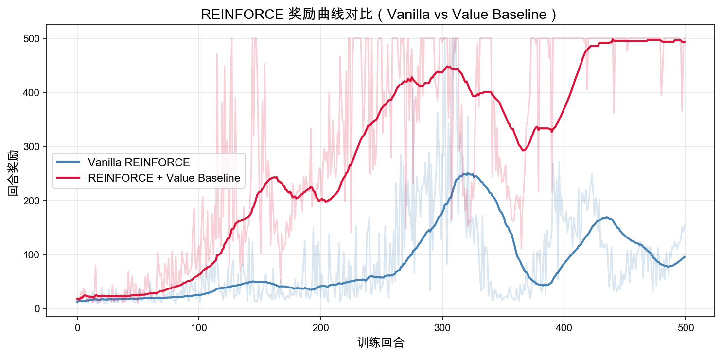
In the plot, the light-colored curve is the raw return of each episode, and the dark curve is a moving average. Large per-episode jumps are normal in policy-gradient problems: under the same policy, different initial conditions can lead to very different episode lengths. For that reason, the moving average trend is more informative than the raw curve.

In this run, the average return over the last 50 episodes for vanilla REINFORCE is about 95.1. It is clearly learning, but it learns slowly, and there is a noticeable mid-training drop. With a value baseline, the average return over the last 50 episodes is about 493.0, which is already very close to CartPole's 500-step limit.

This difference makes the point concrete: the value baseline is not a decorative mathematical term. On the same task, it can bring the policy into the “basically balancing” regime faster, and it reduces the probability of sudden regressions late in training.

5.3.5 Watching the Replays

Reward curves describe average trends; replays show what the policy is actually doing. The two GIFs below are generated by the same rendering script, and they show the deterministic behavior of the two policies after 500 training episodes.

Vanilla REINFORCE: it can survive for a while, but it still tends to drift into instability. In this rendering, the return is 166. The policy is no longer random, but its corrections are not stable enough after the pole starts to deviate; the cart gradually pushes the system into an unrecoverable region.

REINFORCE + Value Baseline: it more consistently pulls the pole back toward the center. In this rendering, the return is 355. It does not hit the 500-step ceiling every time, but its corrective actions are visibly more coherent, and it is more likely to recover when the pole deviates.

The purpose of these replays is not to claim that one particular random seed will always look like this. Rather, they help interpret the gap seen in the reward curves. With the vanilla update, the learning signal is noisier: the policy can pick up useful actions, but its judgment across different states can remain unstable. By using $G_t-V(s_t)$, the Value Baseline version filters out part of the effect of “this state was already easy” or “this state was already dangerous,” and makes it easier for learning to focus on the incremental contribution of the action itself.

5.3.6 Reading the Variance Curves

The reward curve answers, “Is the policy getting better?” The variance curve addresses a different question: why does the value baseline make training more stable?

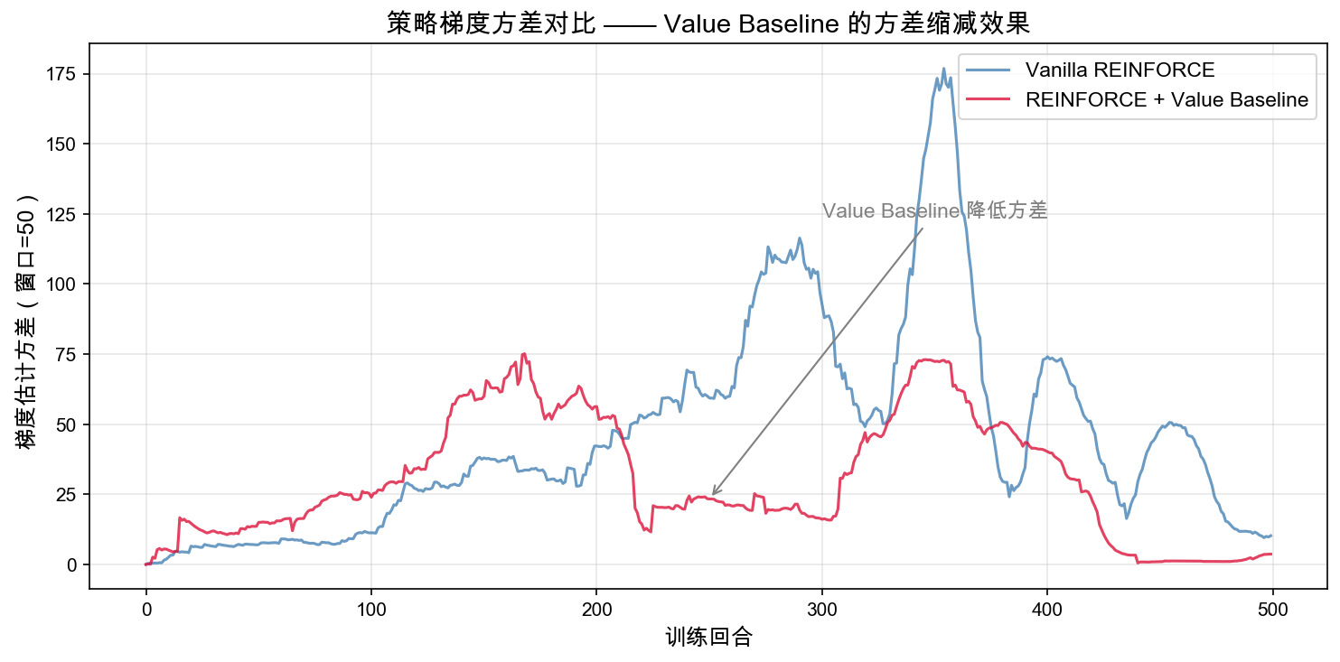
This plot shows the variance of gradient estimates within a sliding window. A larger value means that different episodes imply more divergent update directions; a smaller value means that updates are more consistent from episode to episode.

In this run, the variance of the gradient estimate is about 100.41 for vanilla REINFORCE and about 38.27 for the Value Baseline version. In other words, the Value Baseline reduces the variance to roughly 38.1% of the original. This aligns with what we saw in the reward curves: when the learning signal is steadier, the policy is more likely to keep moving in the direction of “keeping the pole upright.”

5.3.7 What Actually Changed in the Code?

The core update in vanilla REINFORCE is:

returns_t = torch.FloatTensor(returns)
log_probs = torch.log(action_probs + 1e-8)
loss = -(log_probs * returns_t).mean()

Here, returns_t is $G_t$. If an episode happens to last a long time, then all actions along that trajectory are reinforced with a large weight. This is not always wrong, but it tends to reinforce many actions that were merely “not catastrophic yet.”

With a value baseline, the script adds a value network:

values = value_net(states_t)
value_loss = nn.MSELoss()(values, returns_t)

The value network learns: starting from state $s_t$, how many points one typically obtains. Then the policy network no longer uses $G_t$ directly; instead it uses the advantage:

with torch.no_grad():
    values_pred = value_net(states_t)

advantages = returns_t - values_pred
policy_loss = -(log_probs * advantages).mean()

These lines are the essence of the value baseline. If advantages is positive, the outcome was better than expected and the corresponding action should become more likely; if advantages is negative, the outcome was worse than expected and the corresponding action should become less likely.

Note that the value baseline does not depend on the current action itself, and therefore it does not change the expected direction of the policy gradient. What it changes is the magnitude of the estimation noise. This is why we call it “variance reduction,” not “changing the objective.”

5.3.8 Returning to the Picture

Imagine that the cart has already brought the pole close to upright. If from this state it can typically survive for a long time, then surviving a few more steps does not necessarily mean that the previous action was exceptionally good; it may simply reflect that the state is easy. In this case, $V(s_t)$ is large, and after subtracting it, the advantage will not be exaggerated.

Conversely, if the pole is already leaning noticeably and the cart manages to save the episode via a correct action, the realized return may be substantially higher than what the value network expected. Then $G_t-V(s_t)$ is positive, and the policy more clearly reinforces that recovery action.

This is the key sense in which a value baseline is finer than “only looking at the total score”: even if the return is the same, the meaning differs. Scoring 100 points from a dangerous state and scoring 100 points from an easy state are not the same event.

5.3.9 Common Misreadings

Misreading 1: A value baseline makes rewards larger. The value baseline does not change the environment reward. CartPole still gives +1 per time step. What changes is how we interpret those rewards during training.

Misreading 2: A larger baseline is always better. If the baseline estimate is poor, the advantage will also be noisy. We use a value network to learn $V(s)$ because different states have different reasonable expected returns. A fixed constant baseline can only help in very simple, stateless settings.

Misreading 3: With a value baseline, it is already Actor-Critic. This section still uses REINFORCE with a Value Baseline. We must wait until the end of the episode and update using Monte Carlo returns $G_t$. In the next chapter, Actor-Critic will go one step further: it will replace full returns with TD targets so that updates can be performed at every step.

Summary

• CartPole is better than bandits for demonstrating value baselines: it has state, clear failure modes, and episode length makes performance easy to read.
• Vanilla REINFORCE updates with $G_t$, so it is easily misled by episodic luck.
• A Value Baseline learns $V(s_t)$ and changes the learning signal from $G_t$ to $G_t-V(s_t)$.
• The Value Baseline does not change the expected direction of the policy gradient, but it can greatly reduce variance and make training more stable.
• In this section, the baseline already has a “critic-like” flavor; the next chapter turns it into a true Actor-Critic method.

Exercises

1. Change num_episodes to 200 and compare which method reaches a usable policy earlier.
2. Change the learning rate from 1e-3 to 5e-4 or 2e-3 and see whether the Value Baseline remains more stable.
3. Print advantages.mean() and advantages.std() in the script and check whether the advantage signal fluctuates around 0.
4. Reduce the hidden size of the Value Network from 128 to 32 and see whether weaker baseline estimation leads to a noisier training curve.

References

---

1. Williams, R. J. (1992). Simple statistical gradient-following algorithms for connectionist reinforcement learning. Machine Learning, 8, 229-256. DOI: https://doi.org/10.1007/BF00992696. ↩︎

2. Sutton, R. S., McAllester, D., Singh, S., & Mansour, Y. (1999). Policy gradient methods for reinforcement learning with function approximation. Advances in Neural Information Processing Systems, 12. ↩︎

3. Greensmith, E., Bartlett, P. L., & Baxter, J. (2004). Variance reduction techniques for gradient estimates in reinforcement learning. Journal of Machine Learning Research, 5, 1471-1530. https://jmlr.org/papers/v5/greensmith04a.html. ↩︎