27.1 Visual Generation and DanceGRPO

In earlier chapters we started with LLM text post-training: the model reads a piece of text and generates a reply, and the RL objective is to make that reply match human preferences more closely, reason better, and make fewer formatting or factual mistakes. Once we moved into this chapter's predecessor, we expanded the input from pure text to images plus text and talked about the understanding side of VLMs: the model looks at an image, answers a question, and the RL objective is to make it look more accurately and answer more reliably.

Now we take one more step forward, to the other side of visual AI: generation. Give the model a piece of text, and it has to produce an image, or a video.

On the surface this looks like "make the model draw prettier pictures." But in real applications, users rarely want just "pretty." What they actually want is: the right subject, the right count, the right spatial relationships, the right details, and an overall style that looks natural.

For example, suppose the prompt says:

A glass corridor with three red umbrellas; a blue signboard on the wall to the right.

The model generates a beautiful glass corridor, but with only two umbrellas, and the signboard isn't blue. Should this image get a high score or a low one? Judged purely on aesthetics it might score well; judged on instruction following it clearly fails.

So the core problem of visual generation RL is:

Can "generating well" be broken down into a feedback signal that can be learned, compared, and optimized?

This section follows one complete generation trajectory from start to finish: first we look at why visual generation is harder to write a reward for than visual question answering, then we translate the diffusion denoising process into an MDP, and finally we work through DDPO's policy gradient, its training procedure, and its reward model design.

Figure 1: RL post-training results shown in the DDPO paper/project. Different rewards push the diffusion model toward different generation preferences, illustrating the key point of visual generation RL directly: reward design directly shapes the final image distribution. Source: DDPO GitHub, corresponding to Black et al., 2024

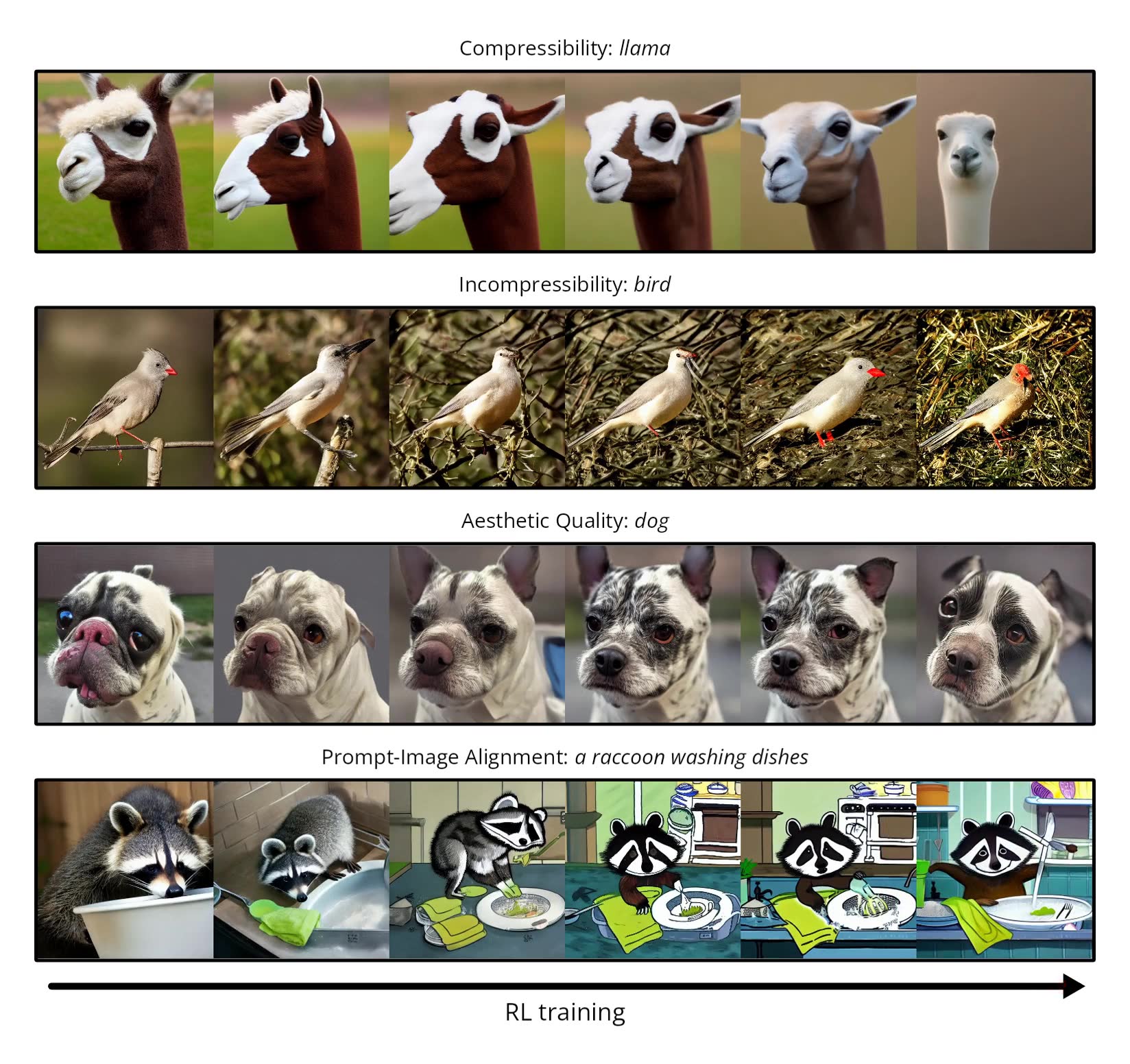
The main algorithmic thread behind this figure comes from the DDPO paper. Later, when we write diffusion as an MDP and update the denoising trajectory with a policy gradient, this paper remains our core reference^[1].

From LLM to VLM to Visual Generation — What Actually Changes When RL Moves Over?

The better way to frame this isn't "can VLM techniques be transplanted directly into generation," but to first lay out a longer route:

LLM text RL → VLM understanding RL → visual generation RL

All three stages use the same basic language of RL: the model is a policy, the model's output forms a trajectory, a reward evaluates that trajectory, and during training KL penalties, clipping, or advantage estimates keep the update stable. But with every step forward, the object being optimized changes.

Start with LLMs. An LLM's input is a text context and its output is text too. One reply can be seen as a token trajectory:

$$y=(y_1,y_2,\dots ,y_T)$$

Each action is "pick the next token." The reward can come from a human-preference model, a rule check, a math verifier, code execution results, or a formatting constraint. PPO, DPO, and GRPO differ in the details, but mostly revolve around "how to make text replies match the reward better."

On the VLM understanding side, the input gains an image:

$$c=(\text{image},\text{text prompt})$$

But the output of many tasks is still text, a multiple-choice option, coordinates, or a bounding box. In other words, the model has more visual evidence to work with, but the action still often lands on a token or a structured answer. The reward is also relatively easy to write: is the answer correct, is the box aligned, is IoU high enough, does the reasoning format satisfy the requirements. This is the core idea behind the VLM-R1 / VISTA-Gym style of work covered in earlier sections: get the model to actually use visual evidence, instead of guessing the answer from language priors alone.

Move on to visual generation, and things genuinely jump to a different level. The model's goal is no longer "look at the image and answer" but "create a new visual result from the prompt." The output is no longer a string of answer tokens — it's an image, a video, or more precisely, a latent / denoising trajectory. The reward here no longer mainly asks "does the answer equal the ground truth," it asks:

• Does the image match the prompt?
• Are the count, colors, and spatial relationships correct?
• Do humans prefer this result?
• Does the image look natural, sharp, and stylistically consistent?
• In a video, are consecutive frames coherent?

We can put these three stages into one table:

Stage	Input	Output	RL's action	What the reward looks like
LLM text post-training	text prompt	text reply	next token	preference, rule, verifier
VLM understanding post-training	image + text question	text, option, box, coordinates	mostly still token or structured answer	answer correctness, IoU, tool verification
Visual generation post-training	text / image condition	image, video, latent trajectory	each step of the denoising transition	preference, alignment, quality, fine-grained constraints

So visual generation RL isn't overturning what came before — it's carrying the same RL language over to a harder object.

What can be inherited: policy gradient, advantage, KL regularization, PPO-style clipping, reward models, judge models. What genuinely has to be rewritten: state, action, trajectory, and reward.

This is exactly why work like DDPO starts with something that looks deceptively simple but is actually essential: translating the diffusion denoising process into states, actions, trajectories, and rewards^[1:1]. Only once this translation is clear do we know exactly what the policy gradient is updating.

Starting from the Diffusion Sampling Process

The generation process of a diffusion model can be understood as "starting from noise and gradually denoising."

At the very start, the model has a latent that is close to pure random noise, denoted $x_T$. The model then generates step by step:

$$x_T\to x_{T-1}\to \cdots \to x_1\to x_0$$

Here $x_0$ is the latent corresponding to the final image. After passing through a decoder, we get the image the user actually sees.

At each denoising step, the model looks at three things:

Symbol	Meaning
$x_t$	the current still-noisy latent
$t$	the current denoising step
$c$	the prompt or condition information

What the model has to decide is the next latent:

$$x_{t-1}\sim p_{\theta }(x_{t-1}\mid x_t,t,c)$$

This line reads: given the current noisy state $x_t$, timestep $t$, and prompt $c$, the model defines a probability distribution with parameters $\theta$ and samples the next step $x_{t-1}$ from it.

Why does this look like a policy? Because in RL, a policy is defined as:

$${\pi }_{\theta }(a\mid s)$$

That is, "given the current state $s$, the probability distribution over choosing action $a$."

We're already familiar with this shape from LLMs:

$${\pi }_{\theta }(y_t\mid y_{<t},c)$$

Given the preceding tokens $y_{<t}$ and context $c$, the model chooses the next token $y_t$. So the token is the action, and the text context is the state.

The diffusion denoising distribution has exactly the same shape:

$$p_{\theta }(x_{t-1}\mid x_t,t,c)$$

Given the current noisy latent, timestep, and prompt, the model chooses the next latent. So we can treat $(x_t,t,c)$ as the state, and $x_{t-1}$, or equivalently the denoising direction, as the action.

Of course, this only says the sampling process can be formally viewed as a policy. It doesn't mean we've already turned it into RL. Only once we define a reward on the final image and use that reward to update $p_{\theta }$ does this sampling process actually become a reinforcement learning problem.

Translating Diffusion into MDP Language

DDPO's (Denoising Diffusion Policy Optimization) key observation is that the diffusion sampling process can be viewed as a finite-horizon MDP. Black et al.'s DDPO paper explicitly frames denoising as a multi-step decision-making problem, then optimizes a downstream reward directly with policy gradient^[1:2].

This translation matters a great deal. Let's go through it term by term:

RL concept	Diffusion counterpart
state $s_t$	the current latent, timestep, and prompt: $(x_t,t,c)$
action $a_t$	sampling the next latent, or predicting the denoising direction
trajectory $\tau$	the full denoising chain: $x_T,\dots ,x_0$
reward $R$	the score given to the final image by a reward model
policy ${\pi }_{\theta }$	the diffusion model's denoising distribution $p_{\theta }$

So one act of generation is like an episode:

$$\tau =(x_T,x_{T-1},\dots ,x_0)$$

In RL, an episode refers to one complete interaction: starting from an initial state, the agent picks actions in sequence, the environment returns the next state each time, and this continues until the task terminates. In CartPole, for instance, the span from when the cart and pole are initialized to when the pole falls or the maximum number of steps is reached is one episode. In text generation, the span from the start token to the end token can also be treated as one episode.

The point of an episode is that it draws a boundary around "the outcome." It tells us which states and actions belong to the same attempt, and which sequence of decisions the final judgment should look back on. For image generation, it's very hard to judge whether any single intermediate latent is "a good image" in isolation. What can actually be scored by a human preference model, a CLIP score, an aesthetic model, or a task reward is usually the final $x_0$. So we treat the entire chain from pure noise $x_T$ denoised step by step down to $x_0$ as one episode, with the terminal state being the final image.

Only after the episode ends does the reward model see the final image and produce a score:

$$R=r_{\varphi }(x_0,c)$$

Note that $r_{\varphi }$ here is not the generative model itself — it's a separate scoring model. Its parameters are $\varphi$, while the generative model's parameters are $\theta$.

With this, the generative model's objective can be written as:

$$J(\theta )={\mathbb{E}}_{\tau \sim p_{\theta }}\left[r_{\varphi }(x_0,c)\right]$$

This reads: we want the average reward of the final image, over trajectories sampled by the model itself, to be as high as possible.

Updating the Denoising Policy with Policy Gradient

With the MDP translation above, DDPO stops being mysterious. At its core it's just policy gradient applied to diffusion sampling trajectories.

Let's first give this derivation its paper coordinates. On the left of the table is what we're about to do; on the right is the classic line of work it comes from.

What we're about to do	Corresponding paper lineage
Treat one act of denoising generation as an episode / MDP	DDPO: Black et al., 2024[1:3]
Raise the probability of high-scoring samples and lower it for low-scoring ones; mathematically, this is a policy gradient	REINFORCE: Williams, 1992[2]
Use an old/new logprob ratio with clipping so each update doesn't take too large a step	PPO: Schulman et al., 2017[3]
Use a KL constraint to keep the model from drifting too far from a reference model	DPOK: Fan et al., 2023[4]
Train a reward model on human or aesthetic preference	Pick-a-Pic / HPS v2[5][6]

The row most likely to be intimidated by its own terminology is the second one. In plain language it's simple:

If a denoising trajectory ends up producing a high-scoring image, make the model more likely to sample the steps in that trajectory going forward; if it scores low, make those steps less likely to be sampled.

The catch is that training a model can't just be told "make this more likely to happen." We need a computable gradient direction. The log-derivative trick in REINFORCE is exactly the step that turns this sentence into a trainable formula.

Let's first align the notation we'll use going forward:

Symbol	How to think about it for now
$\theta$	the diffusion model's parameters — what training actually changes
$c$	the prompt
$\tau$	one full generation trajectory, denoised from $x_T$ down to $x_0$
$p_{\theta }(\tau )$	the probability the current model assigns to sampling this trajectory
$R(\tau ,c)$	the score given to the image this trajectory ultimately produces
$J(\theta )$	the current model's average score; the training objective is to make this larger
${\nabla }_{\theta }$	the direction in which changing the parameters makes $J(\theta )$ larger — the gradient

Let's first write out the probability of a full denoising trajectory. To simplify notation, we assume below that the prompt $c$ is given:

$$p_{\theta }(\tau \mid c)=p(x_T)\prod _{t=1}^T{p}_{\theta }(x_{t-1}\mid x_t,t,c)$$

This line carries two meanings.

First, the initial noise $x_T$ is normally sampled from a standard Gaussian, and it does not depend on the model parameters $\theta$. Second, what the model actually controls is each step's denoising distribution $p_{\theta }(x_{t-1}\mid x_t,t,c)$.

The product form is intuitive too: for a whole trajectory to occur, step $T$ has to sample $x_{T-1}$, step $T-1$ has to sample $x_{T-2}$, and so on until $x_0$ is finally sampled. So the probability of the whole trajectory is the product of the probabilities at every step.

The generative model wants to maximize the final reward:

$$J(\theta )={\mathbb{E}}_{\tau \sim p_{\theta }(\tau \mid c)}\left[R(\tau ,c)\right]$$

where $R(\tau ,c)=r_{\varphi }(x_0,c)$, i.e., the reward model's score for the final image.

Let's first build intuition with a discrete toy example. Suppose that under the same prompt, the model can only sample three possible denoising trajectories:

Trajectory	Probability the model samples it	Final reward
${\tau }_1$	$p_1$	$R_1$
${\tau }_2$	$p_2$	$R_2$
${\tau }_3$	$p_3$	$R_3$

Then the average reward is:

$$J=p_1{R}_1+p_2{R}_2+p_3{R}_3$$

If ${\tau }_2$'s reward is high, we naturally want $p_2$ to increase. In other words, the intuition of an RL update isn't "push the pixels of the image directly in some direction" — it's "change the model's sampling probabilities": push the probability of high-scoring trajectories up, and push the probability of low-scoring trajectories down.

A real diffusion model doesn't just have three trajectories — it has a continuous, enormous space of possible trajectories. Writing the weighted average above as an integral gives:

$$J(\theta )=\int p_{\theta }(\tau \mid c)R(\tau ,c)d\tau$$

There's no need to be intimidated by this integral. It's just "multiply the probability of every possible trajectory by its score, and add them all up." In the discrete case that's $p_1{R}_1+p_2{R}_2+p_3{R}_3$; in the continuous case, it's written as an integral.

Now take the gradient with respect to $\theta$ — that is, ask: in which direction should the model parameters change to make the average reward go up?

$${\nabla }_{\theta }J(\theta )=\int {\nabla }_{\theta }{p}_{\theta }(\tau \mid c)R(\tau ,c)d\tau$$

Here's the problem: this expression contains ${\nabla }_{\theta }{p}_{\theta }(\tau \mid c)$, meaning "how does the probability of this entire trajectory change as the model parameters change." But during training, what we actually get is a batch of trajectories sampled from the model — we can never enumerate every possible trajectory. We want to rewrite the gradient as an "average over sampled trajectories" so it can be estimated from actual samples.

This is where a very small identity comes in, called the log-derivative trick, also known as the score-function trick. It's exactly the core technique behind REINFORCE-style policy gradient methods^[2:1]:

$${\nabla }_{\theta }{p}_{\theta }(\tau \mid c)=p_{\theta }(\tau \mid c){\nabla }_{\theta }\log p_{\theta }(\tau \mid c)$$

This identity just rewrites $\nabla p$ as $p\nabla \log p$. Here's why:

$${\nabla }_{\theta }\log p_{\theta }=\frac{1}{p_{\theta }}{\nabla }_{\theta }{p}_{\theta }$$

Multiplying both sides by $p_{\theta }$ gives:

$$p_{\theta }{\nabla }_{\theta }\log p_{\theta }={\nabla }_{\theta }{p}_{\theta }$$

It sounds like a trick, but it's really just an algebraic rewrite. Its benefit is that $p_{\theta }(\tau \mid c)$ reappears in the formula, and that's exactly what "sampling a trajectory from the current model" represents. So we can now estimate the gradient using trajectories we actually sampled.

Substituting back:

$${\nabla }_{\theta }J(\theta )=\int p_{\theta }(\tau \mid c){\nabla }_{\theta }\log p_{\theta }(\tau \mid c)R(\tau ,c)d\tau$$

That is:

$${\nabla }_{\theta }J(\theta )={\mathbb{E}}_{\tau \sim p_{\theta }}\left[{\nabla }_{\theta }\log p_{\theta }(\tau \mid c)R(\tau ,c)\right]$$

This step matters a great deal, because it turns an intractable problem into one that can be estimated by sampling. During training we only need to do three things:

1. Sample a trajectory $\tau$ from the current diffusion model;
2. Use the reward model to score the final image, getting $R(\tau ,c)$;
3. Look at this trajectory's log probability under the model, i.e., $\log p_{\theta }(\tau \mid c)$, and push it up or down depending on how high or low the reward was.

So the policy gradient never needs to differentiate through the reward itself. The reward model can be non-differentiable, or even a black-box scorer — all we need is "how many points did this trajectory get." This is exactly the property DDPO exploits: the reward can come from an aesthetic model, a compression ratio, VLM feedback, or any other objective that can't be directly backpropagated through^[1:4].

Next, expand the trajectory's log probability:

$$\log p_{\theta }(\tau \mid c)=\log p(x_T)+\sum _{t=1}^T\log p_{\theta }(x_{t-1}\mid x_t,t,c)$$

Why take the log? Because the original trajectory probability is a long product of probabilities. A long product is hard to work with; once we take the log, multiplication turns into addition:

$$\log (ab)=\log a+\log b$$

So the log probability of the whole trajectory equals the sum of the log probabilities at every step.

Since $\log p(x_T)$ doesn't depend on $\theta$, it drops out when we take the gradient:

$${\nabla }_{\theta }\log p_{\theta }(\tau \mid c)=\sum _{t=1}^T{\nabla }_{\theta }\log p_{\theta }(x_{t-1}\mid x_t,t,c)$$

So the most basic form of the policy gradient is:

$${\nabla }_{\theta }J=\mathbb{E}\left[\sum _{t=1}^T{\nabla }_{\theta }\log p_{\theta }(x_{t-1}\mid x_t,t,c)\cdot R(\tau ,c)\right]$$

This is REINFORCE's form on a diffusion trajectory^[2:2]: if a denoising trajectory ends up with a high reward, raise the sampling probability of every step in that trajectory; if the reward is low, lower them. Black et al.'s DDPO paper is exactly this idea carried over to diffusion's denoising trajectories^[1:5].

Why Can We Subtract a Baseline and an Advantage?

Updating directly with $R(\tau ,c)$ has very high variance. One prompt might naturally be easier to generate high-scoring images for, while another might naturally be harder. What we actually care about is: is this particular sample better than similar samples?

So we can subtract a baseline $b(c)$:

$$\hat{A}=R(\tau ,c)-b(c)$$

Here $\hat{A}$ is called the advantage. It doesn't ask "what is this image's absolute score" — it asks "how much better is it than the reference level." If the reward is 8 and the baseline is 6, the advantage is +2, meaning this generation was better than expected; if the reward is 5 and the baseline is 6, the advantage is -1, meaning this generation was worse than expected.

Why is it legitimate to subtract a baseline? The intuition: if you subtract the same constant from every score in the same group of samples, which one is better than which doesn't change. What training actually needs is "relatively better" or "relatively worse."

Mathematically we can also verify this doesn't change the expected gradient. All we need to show is that, on average, the term that gets subtracted off equals zero.

$${\mathbb{E}}_{\tau \sim p_{\theta }}\left[{\nabla }_{\theta }\log p_{\theta }(\tau \mid c)b(c)\right]=b(c)\int p_{\theta }(\tau \mid c){\nabla }_{\theta }\log p_{\theta }(\tau \mid c)d\tau$$

We can pull $b(c)$ outside because, for a fixed prompt, it's a constant that doesn't depend on the specific sampled action. Applying the same log-derivative trick again:

$$=b(c)\int {\nabla }_{\theta }{p}_{\theta }(\tau \mid c)d\tau =b(c){\nabla }_{\theta }\int p_{\theta }(\tau \mid c)d\tau =b(c){\nabla }_{\theta }1=0$$

Why is the last line 1? Because $\int p_{\theta }(\tau \mid c)d\tau$ represents "the probabilities of all possible trajectories added up," and probabilities must sum to 1. The gradient of a constant 1 with respect to the parameters is 0. So subtracting a baseline that doesn't depend on the specific action doesn't change the average update direction — it only makes the update more stable.

In actual training, $\hat{A}$ is commonly computed in a few different ways:

Advantage formula	Meaning
$R-\bar{R}$	subtract the mean reward of the same batch
$R-b(c)$	subtract the prompt-level historical average reward
$R-V_{\psi }(x_t,t,c)$	subtract a value model's prediction for the current state
normalized reward	standardize the batch reward to stabilize the scale

With the advantage added in, the policy gradient DDPO commonly uses can be written as:

$${\nabla }_{\theta }J=\mathbb{E}\left[\sum _{t=1}^T{\nabla }_{\theta }\log p_{\theta }(x_{t-1}\mid x_t,t,c)\cdot {\hat{A}}_t\right]$$

If we only use the terminal reward, every step can share the same $\hat{A}$. If a value model is trained, different timesteps can get different ${\hat{A}}_t$.

How Does This Map onto Diffusion's Log Probability?

In many diffusion implementations, each reverse transition step can be written as a Gaussian distribution:

$$p_{\theta }(x_{t-1}\mid x_t,t,c)=\mathcal{N}\left({\mu }_{\theta }(x_t,t,c),{\sigma }_t^{2}I\right)$$

Here ${\mu }_{\theta }$ is the denoising mean predicted by the model, and ${\sigma }_t$ is the noise scale at this step. DDPO's implementation needs to record the log probability of each step's action, which essentially means taking the logprob under this reverse transition distribution^[1:6]. So the log probability of this action is approximately:

$$\log p_{\theta }(x_{t-1}\mid x_t,t,c)=-\frac{1}{2{\sigma }_t^2}{\Vert x_{t-1}-{\mu }_{\theta }(x_t,t,c)\Vert }_2^2+\text{const}$$

This line's meaning is also simple: if the actually sampled $x_{t-1}$ is close to the model's predicted mean ${\mu }_{\theta }(x_t,t,c)$, the squared distance is small and the log probability is high; if it's far away, the squared distance is large and the log probability is low.

This explains what step.logprob in the pseudocode is: it isn't an abstract RL symbol — it's literally the log probability that the current model assigned to sampling this particular $x_{t-1}$ at step $t$.

From Maximizing an Objective to Minimizing a Loss

Deep learning frameworks typically minimize a loss, while policy gradient is maximizing $J(\theta )$. So in the implementation this is flipped with a negative sign:

$${\mathcal{L}}_{\text{pg}}=-\mathbb{E}\left[\sum _{t=1}^T\log p_{\theta }(x_{t-1}\mid x_t,t,c)\cdot {\hat{A}}_t\right]$$

Minimizing this loss is equivalent to maximizing the policy gradient objective. Intuitively:

Case	What the loss pushes toward
${\hat{A}}_t>0$	raise the log probability of this step's sampled action
${\hat{A}}_t<0$	lower the log probability of this step's sampled action
${\hat{A}}_t\approx 0$	leave this step essentially unchanged

This is exactly the same idea as REINFORCE from Chapter 5 — only the action has changed from "pick a token" to "pick the next latent."

Why Do We Still Need a KL Constraint?

If we only maximize reward, the model easily goes off the rails. The reason is simple: the reward model itself is never perfect. The model can discover patterns the reward model happens to like, but that humans don't actually like.

So in practice, training usually keeps a reference model $p_{\text{ref}}$ around, and penalizes the current model for drifting too far from it. DPOK also treats "policy optimization + KL regularization" as the core structure of text-to-image diffusion RL fine-tuning^[4:1]:

$${\mathcal{L}}_{\text{DDPO}}={\mathcal{L}}_{\text{pg}}+\beta \mathbb{E}\left[\sum _{t=1}^T\mathrm{KL}\left(p_{\theta }(\cdot \mid x_t,t,c)\Vert p_{\text{ref}}(\cdot \mid x_t,t,c)\right)\right]$$

This expression breaks into two parts:

Term	Role
policy gradient term	makes high-reward sampled trajectories more likely to occur
KL term	keeps the model from chasing reward so hard that it drifts away from the original model

This is the same idea as in RLHF, DPO, and GRPO: make the model better, but don't fly the model off the rails.

DDPO's Minimal Training Loop

The derivation above explains "why we're allowed to update." Now let's break down the training process to see clearly how data flows from prompt to loss in a single DDPO update.

Start with one sentence worth remembering:

DDPO isn't supervised learning on existing images — it lets the current model generate images itself, uses reward to judge whether those generations are good, and finally routes that good/bad signal back onto the sampling trajectory^[1:7].

This is also the core difference from ordinary diffusion fine-tuning. Ordinary supervised fine-tuning shows the model "what it should generate." DDPO shows the model "among the results you generated yourself, which ones deserve to become more likely."

Step 1 — Take a Batch of Prompts

The first step isn't taking images — it's taking prompts:

$$\mathcal{B}=\{c_i{\}}_{i=1}^B$$

where $B$ is the batch size and $c_i$ is the $i$-th prompt.

The quality of the prompt data directly affects the training direction. If the prompts are too simple, the model may only learn to raise its general aesthetic score; if the prompts contain fine-grained constraints on count, color, position, and relationships, the reward model has a chance to actually train the model's instruction-following ability.

In practice, a good prompt batch tends to mix several categories:

Prompt type	Training role
simple-scene prompts	stabilizes baseline generation quality
multi-attribute prompts	trains color, material, count, and other details
spatial-relation prompts	trains left/right, above/below, occlusion, relative position
long-instruction prompts	trains instruction following under complex conditions
evaluation-set-style prompts	keeps the training objective aligned with final evaluation

This step looks mundane but is critical: RL can only optimize the model's behavior over the distribution of these prompts. If the prompt distribution is too narrow, the model can easily improve only within that narrow scenario.

Step 2 — Roll Out with the Current Model

The second step is generating images with the current diffusion model. In RL this step is usually called a rollout — letting the policy run through a trajectory on its own.

For each prompt $c_i$, the model starts from noise $x_T$ and samples an entire denoising chain:

$${\tau }_i=(x_T^{(i)},x_{T-1}^{(i)},\dots ,x_0^{(i)})$$

There's a detail that's easy to overlook here: during training we can't just save the final image — we also need to save key information from every denoising step.

What to save	Why it needs to be saved
$x_t$	needed to recompute this step's log probability later
$x_{t-1}$	this is the action actually sampled at step $t$
$\log p_{{\theta }_{\text{old}}}(x_{t-1}\mid x_t,t,c)$	needed as the old logprob for PPO-style updates later
the final image $x_0$ or decoded image	the reward model needs to score the final result

Why does ${\theta }_{\text{old}}$ show up here? Because when the image was sampled, the model in use was still the pre-update model. By the time we compute a gradient update, the model's parameters are already about to change. To know "how much the new model has changed this step's action probability relative to the old model," we usually need to keep the old logprob around.

If we're only doing one naive REINFORCE update, we can use the logprob from the sampling step directly. But in real training, to improve sample efficiency, the same batch of rollouts is usually reused across multiple update epochs, and that's when the old logprob really matters. This old/new policy ratio idea comes from PPO^[3:1]; the importance-sampling variant used in DDPO also follows this "keep the rollout fixed, then correct the update with a probability ratio" approach^[1:8].

Step 3 — Score the Final Result with a Reward Model

The third step hands the generated image to the reward model:

$$R_i=r_{\varphi }(x_0^{(i)},c_i)$$

There's something worth flagging here: the reward model only needs to score the image — it doesn't necessarily need to participate in backpropagation. What policy gradient needs is "how many points did this trajectory get," not the gradient of the reward with respect to pixels or latents.

This is also one of DDPO's advantages over backpropagating through a differentiable reward. The reward can come from a very complex system — a VLM judge, a human preference model, a rule checker, even a combination of multiple models. As long as it can ultimately produce a scalar score, it can serve as the signal for the policy gradient. By contrast, work like DRaFT and VADER exploits the gradient of a differentiable reward and backpropagates it directly into the image or video diffusion model^[7][8].

A common reward computation pipeline looks like:

1. Decode the latent $x_0$ into an image.
2. Use a text-image alignment model to check whether it matches the prompt.
3. Use a preference model or aesthetic model to score visual quality.
4. Use rules or a VLM to check hard constraints like count, color, and spatial relationships.
5. Combine these into the final reward $R_i$.

The biggest danger here is unstable reward scales. Some rewards might live in $[0,1]$, others in $[-10,10]$; adding them directly lets one term dominate training. So actual training usually applies clipping, normalization, or layered filtering.

Step 4 — Turn Reward into Advantage

The fourth step computes advantage from reward. The simplest approach is batch-wise centering:

$${\hat{A}}_i=R_i-\frac{1}{B}\sum _{j=1}^B{R}_j$$

For an even more stable scale, we can also divide by the standard deviation:

$${\hat{A}}_i=\frac{R_i-\mathrm{mean}(R)}{\mathrm{std}(R)+ϵ}$$

With this, ${\hat{A}}_i>0$ means image $i$ is better than the batch average, and ${\hat{A}}_i<0$ means it's worse than average.

Why not just use $R_i$ directly? Because an absolute score is often hard to interpret. One prompt might be intrinsically hard, so scoring 0.6 is already quite good; another prompt might be easy, so scoring 0.8 might just be average. Advantage cares about "relative performance," which makes training more stable.

In more complete implementations, we can also train a value model:

$$V_{\psi }(x_t,t,c)\approx \mathbb{E}[R\mid x_t,t,c]$$

and then use:

$${\hat{A}}_{i,t}=R_i-V_{\psi }(x_t^{(i)},t,c_i)$$

This lets different timesteps have different advantages. That said, for a first understanding of DDPO, a batch-mean baseline is already enough to capture the core idea.

Step 5 — Compute the Policy Gradient Loss

The fifth step is where the diffusion model actually gets updated.

Let's start with the minimal REINFORCE loss. It does exactly one thing: multiply "this trajectory's log probability" by "how good this trajectory was."

$${\mathcal{L}}_{\text{pg}}=-\frac{1}{B}\sum _{i=1}^B\sum _{t=1}^T\log p_{\theta }(x_{t-1}^{(i)}\mid x_t^{(i)},t,c_i)\cdot {\hat{A}}_i$$

This formula can be read in three layers:

Piece of the formula	Meaning
$\log p_{\theta }(x_{t-1}^{(i)}\mid x_t^{(i)},t,c_i)$	the model's log probability of sampling this denoising action at step $t$
${\hat{A}}_i$	how much better image $i$ is than average
the leading minus sign	because the optimizer minimizes loss by default, but we want to maximize the probability of good trajectories

If ${\hat{A}}_i>0$, this image is better than average, and minimizing the loss raises the log probability of every step's action in this trajectory. If ${\hat{A}}_i<0$, this image is worse than average, and minimizing the loss lowers the log probability of those actions.

Many implementations also use a PPO-style importance ratio. This ratio and the clip objective that follows correspond to the core stabilization design of the PPO paper^[3:2]:

$${\rho }_{i,t}(\theta )=\frac{p_{\theta }(x_{t-1}^{(i)}\mid x_t^{(i)},t,c_i)}{p_{{\theta }_{\text{old}}}(x_{t-1}^{(i)}\mid x_t^{(i)},t,c_i)}=\exp \left(\log p_{\theta }(x_{t-1}^{(i)}\mid x_t^{(i)},t,c_i)-\log p_{{\theta }_{\text{old}}}(x_{t-1}^{(i)}\mid x_t^{(i)},t,c_i)\right)$$

This represents how much the new model has raised the probability of the same denoising action relative to the old model. For instance, $\rho =1.2$ means the new model makes this action roughly 20% more likely; $\rho =0.7$ means the new model makes it less likely. In implementations, this is usually computed by subtracting logprobs and then applying exp, purely because logprobs are more numerically stable and easier to save during sampling.

We can then write down the clipped objective:

$${\mathcal{L}}_{\text{clip}}=-\frac{1}{B}\sum _{i=1}^B\sum _{t=1}^T\min \left({\rho }_{i,t}{\hat{A}}_i,\mathrm{clip}({\rho }_{i,t},1-ϵ,1+ϵ){\hat{A}}_i\right)$$

Clipping's job is to limit how aggressive a single update can be. With $ϵ=0.2$, for instance, the ratio typically gets constrained to around $[0.8,1.2]$. In other words, even if an image gets an extremely high reward, the new model still isn't allowed to blow up the probability of a given action in one shot.

The min in this formula can also be read this way: when the update direction is favorable, it's only allowed to bring bounded gains; once the ratio moves past the clip range, further increasing it doesn't make the objective any better. This stops the model from suddenly shifting because of one small batch of high-scoring samples. Mapped onto diffusion, this is about not letting a single reward update push the denoising distribution too far from the original model; both KL regularization and ratio clipping are there to control exactly this^[3:3][4:2].

Step 6 — Add KL Regularization and Update the Parameters

The last step combines the policy gradient loss, KL regularization, and any other stabilizing terms:

$$\mathcal{L}={\mathcal{L}}_{\text{clip}}+\beta {\mathcal{L}}_{\text{KL}}$$

where:

$${\mathcal{L}}_{\text{KL}}=\frac{1}{B}\sum _{i=1}^B\sum _{t=1}^T\mathrm{KL}\left(p_{\theta }(\cdot \mid x_t^{(i)},t,c_i)\Vert p_{\text{ref}}(\cdot \mid x_t^{(i)},t,c_i)\right)$$

$p_{\text{ref}}$ is usually the base diffusion model from before RL began. It acts as an anchor, keeping the model from drifting too far in pursuit of the reward model's preferences.

We can think of the KL term simply as "the distance between two probability distributions." If the current model's denoising distribution at a given step is close to the reference model's, the KL is small; if the current model has produced a very different distribution in order to chase reward, the KL is large. $\beta$ controls how heavy this penalty is: larger $\beta$ makes the model more conservative; smaller $\beta$ lets the model chase reward more aggressively.

Only at this point does standard backpropagation run:

1. Compute the total loss.
2. Call loss.backward() to get gradients.
3. Clip gradients to avoid explosions.
4. Call optimizer.step() to update the diffusion model.
5. Move on to the next batch of prompts and repeat rollout and update.

Putting all six steps together gives pseudocode much closer to real training. It isn't a line-by-line copy of any particular repository — it puts DDPO's rollout/reward update^[1:9], PPO's clipped objective^[3:4], and the KL constraint DPOK emphasizes^[4:3] into one minimal training loop:

for prompts in prompt_loader:
    # Step 1-2: rollout with the current policy
    with torch.no_grad():
        trajectories = diffusion.sample_trajectories(
            prompts,
            return_states=True,
            return_actions=True,
            return_logprobs=True,
        )
        old_logprobs = trajectories.logprobs
        images = decoder(trajectories.final_latents)

    # Step 3: score final images
    with torch.no_grad():
        rewards = reward_model(prompts, images)

    # Step 4: turn rewards into advantages
    advantages = (rewards - rewards.mean()) / (rewards.std() + 1e-6)

    # Step 5-6: update the diffusion policy
    for _ in range(update_epochs):
        logprobs = diffusion.logprob(
            states=trajectories.states,
            actions=trajectories.actions,
            prompts=prompts,
        )

        ratio = torch.exp(logprobs - old_logprobs)
        unclipped = ratio * advantages[:, None]
        clipped = ratio.clamp(1 - eps, 1 + eps) * advantages[:, None]
        policy_loss = -torch.minimum(unclipped, clipped).mean()

        kl_loss = diffusion.kl_to(reference_model, trajectories, prompts)
        loss = policy_loss + beta * kl_loss

        optimizer.zero_grad()
        loss.backward()
        torch.nn.utils.clip_grad_norm_(diffusion.parameters(), max_norm)
        optimizer.step()

This code adds one engineering detail the math above doesn't spell out: sampling and updating are separate. Sampling uses the old model, so old_logprobs has to be saved; updating recomputes logprobs with the current model, and the ratio tells us how much the new model has changed relative to the old one.

If we compress DDPO into one engineering intuition:

For the same batch of prompts, let the model generate a batch of samples on its own; split the results into good and bad by reward; raise the probability of good samples' denoising trajectories and lower the probability of bad samples' denoising trajectories, while using KL and clipping to keep the model from drifting too aggressively.

The Reward Model — The Real Bottleneck of Generation RL

At this point, we have the algorithm. But the hard part of generation RL usually isn't "can we write down a policy gradient" — it's "can the reward actually be trusted."

If the reward model is too weak, it can't give a useful direction; if the reward model is biased, the generative model learns that bias; if the reward is too complex, different objectives start pulling against each other.

Visual generation rewards typically come from three kinds of signal.

Human Preference

The most common form of human preference data is pairwise comparison. Given the same prompt, a user picks the candidate image they prefer between two options. Pick-a-Pic is the representative public dataset for collecting text-to-image user preferences, and HPS v2 further provides a human-preference-focused evaluation benchmark and a reward model recipe^[5:1][6:1].

Figure 2: Pick-a-Pic's human preference collection interface. Users choose their preferred candidate between two images for the same prompt, and this kind of data can be used to train reward models like PickScore. Source: Stability AI Research, corresponding to Kirstain et al., 2023

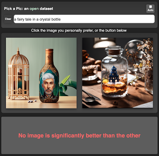
Pick-a-Pic's contribution isn't just its interface screenshots — it's organizing large-scale pairwise text-to-image preference data into a public resource that can actually be trained and evaluated on^[5:2].

Data of this kind can be written as:

$${\mathcal{D}}_{\text{pref}}=\{(c,x^{+},x^{-})\}$$

where $x^{+}$ is the image the user preferred and $x^{-}$ is the one that lost the comparison. The reward model's training objective is typically to make $x^{+}$'s score higher than $x^{-}$'s:

$${\mathcal{L}}_{\text{rm}}=-{\mathbb{E}}_{{\mathcal{D}}_{\text{pref}}}\log \sigma \left(r_{\varphi }(c,x^{+})-r_{\varphi }(c,x^{-})\right)$$

This is Bradley-Terry-style preference modeling. It doesn't require humans to give an absolute score — only to compare two images and say which one is better. Datasets like Pick-a-Pic use exactly this kind of pairwise preference to train or evaluate image preference models^[5:3].

The advantage of this kind of signal is that it's close to genuine user preference. The downside is that it's expensive to collect, and preference data inherits the aesthetics, culture, and task distribution of whoever did the labeling.

Text-Image Alignment

Text-image alignment checks whether the image actually matches the prompt.

This can be broken down from coarse to fine into several layers:

Level	Example	Possible checking method
global semantics	whether the specified scene was roughly generated	CLIP Score, VLM judgment
object presence	whether key objects mentioned in the prompt appear	detector, VLM question answering
attribute match	whether color, material, and size are correct	fine-grained captioning followed by item-by-item comparison
relation match	whether left/right, above/below, occlusion, and interaction relations are correct	relation extraction, VLM judge
count match	whether the specified count is correct	counting model, object detection, VLM check

This layer connects directly to the VLM RL covered in earlier sections. A VLM that's been trained to look at images more carefully can serve as a captioner, judge, or reward model, helping the generative model figure out whether it "got the picture right."

Visual Quality

Visual quality checks whether the image itself looks natural, sharp, and has good composition and lighting. Common signals include aesthetic score, no-reference image quality assessment, and human ranking. Benchmarks like HPS v2 try to turn "which generated result do humans prefer" into a reproducible evaluation and model signal^[6:2].

This is useful, but can't be used on its own. Visual quality models tend to more easily reward images that "look polished" rather than images that "strictly follow the prompt." If a generative model chases only this score, it may become prettier while becoming less obedient.

Reward Isn't a Formula Where More Complexity Is Always Better

Summing all the rewards with weights is a natural instinct:

$$R_{\text{total}}=w_1{R}_{\text{align}}+w_2{R}_{\text{quality}}+w_3{R}_{\text{instruction}}$$

But this formula is only a starting point, not an answer. The biggest problem with multi-component rewards is that every component can be gamed by the model, and the components can conflict with each other.

A more robust engineering approach is to use the reward in layers:

1. First use rules or a VLM to check hard constraints, such as count, color, and whether objects are present.
2. Then use a preference model to rank the samples that pass.
3. Finally use manual spot-checks or offline benchmarks to find the reward model's blind spots.

This way reward stops being one all-purpose score and becomes a filtering-and-calibration pipeline instead.

Figure 3: PickScore re-ranking candidate generations with a preference model. This illustrates that a visual reward isn't just an offline evaluation number — it can also directly change which result is shown to the user during sampling or ranking. Source: Stability AI Research

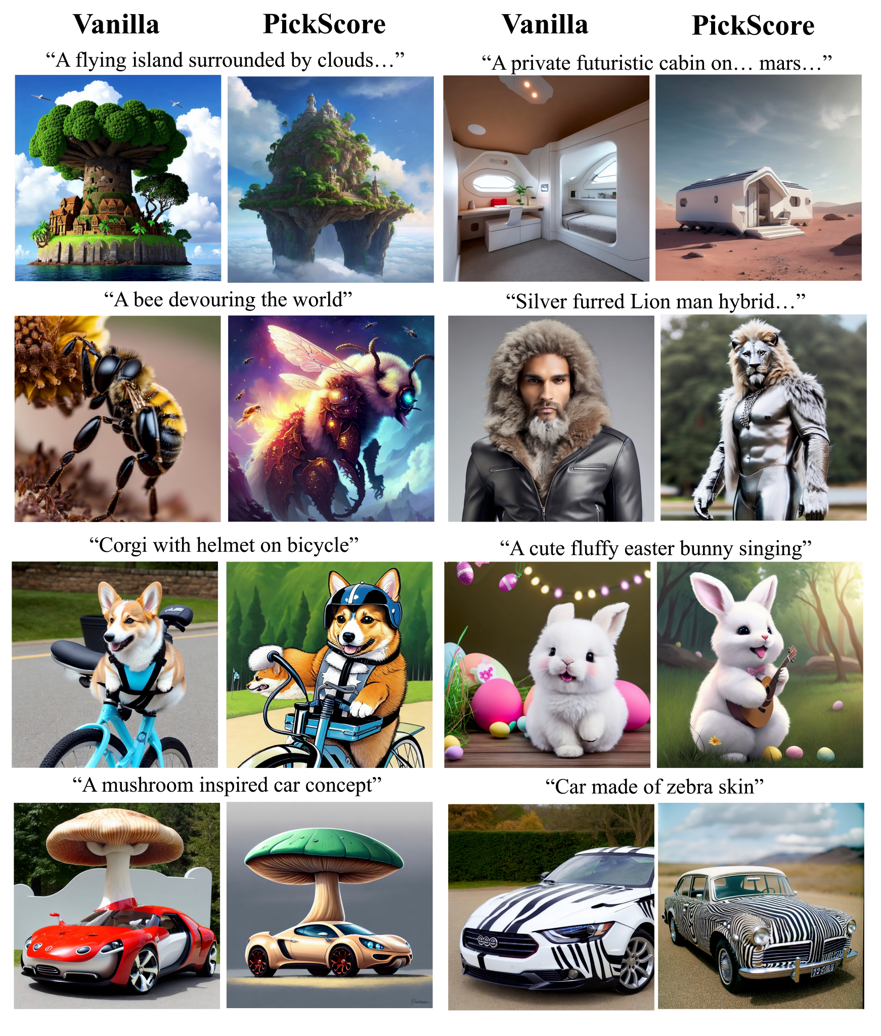
Two Ways to Use a Reward — At Training Time, or at Inference Time?

Once we have a reward model, RL fine-tuning isn't the only option. There are two common ways to use it.

The first is using it at inference time, also called reward-guided sampling or reranking. For example, generate $N$ images for the same prompt, rank them with the reward model, and pick the highest-scoring one. This method is simple and safe, and it's a good way to first check whether the reward model is actually trustworthy.

The second is using it at training time — this is where RL fine-tuning approaches like DDPO and DPOK come in^[1:10][4:4]. The model isn't just being filtered — its parameters are genuinely updated, internalizing the preference into the generation policy itself.

Method	What it does	Advantage	Disadvantage
Best-of-$N$ / reranking	generate several extra images, then pick with the reward model	simple to implement, doesn't touch the model	expensive at inference time, capability isn't internalized
Reward-guided sampling	use the reward to steer direction during sampling	more proactive than pure reranking	still needs extra evaluation on every generation
RL fine-tuning	update the model's parameters with reward	internalizes preference	training is more expensive and easier to destabilize

In practice, teams usually start with reranking. If the reward model can't even rank samples well, it shouldn't be used for RL directly.

The Same Problem, With an Extra Time Axis

Video generation can be seen as an extension of image generation, but it shouldn't be understood simply as "generate a few more images." Video adds a time axis, so the reward needs an extra layer too. Emu Video is an example of work that models image conditioning and video generation as separate factors^[9]; subsequent video alignment work has started exploring reward gradients or MLLM feedback to optimize video generation results^[8:1][10].

A video has to satisfy three things at once:

1. Every frame has to be sharp, natural, and consistent with the prompt.
2. Adjacent frames have to be coherent — the subject can't suddenly change.
3. The whole video has to express the sequence of events described in the prompt.

So video reward is often written in this kind of layered form. This isn't a fixed formula from any specific paper — it's an abstraction of three common categories of evaluation signal (per-frame quality, temporal consistency, and overall event alignment) folded into a single reward:

$$R_{\text{video}}=\alpha \cdot \frac{1}{T}\sum _t{R}_{\text{frame}}(x_t,c)+\beta \cdot \frac{1}{T-1}\sum _t{R}_{\text{temporal}}(x_t,x_{t+1})+\gamma \cdot R_{\text{overall}}(\{x_t{\}}_{t=1}^T,c)$$

These three components correspond to:

Component	What it checks
$R_{\text{frame}}$	per-frame quality and per-frame text alignment
$R_{\text{temporal}}$	inter-frame consistency and motion naturalness
$R_{\text{overall}}$	whether the whole video accomplishes the prompt's event

The challenges of video RL grow accordingly:

Challenge	Why it's harder	Common mitigations
temporal consistency	every frame being good doesn't mean they cohere together	optical-flow consistency, trajectory consistency, video-VLM evaluation
long horizon	far more video tokens/latents than a single image	segment-wise optimization, short-clip reward shaping
compute cost	every sampling-and-scoring pass is more expensive	latent-space training, low frame-rate evaluation, candidate reranking
text-video alignment	the prompt may specify an event order	segment-level captioning, event-level reward

Intuitively, an image generation error is usually "something was drawn wrong somewhere"; a video generation error is usually "the continuity between moments broke down." That's why video reward leans more heavily on segment-level and overall-level evaluation.

On-Policy Distillation — Locking in the Capability RL Produced

An RL-fine-tuned model may match preferences better, but it can also become slower, more expensive, or only suited to one particular sampling setup. The goal of on-policy distillation is to take the high-quality samples an RL-trained model produces on its current distribution, and turn them back into a cheaper supervised learning signal.

This can be understood as three steps:

1. Use the RL-trained teacher model to generate samples online.
2. Filter to keep high-quality samples, using the reward model or rules.
3. Have a student model learn from these samples, reproducing the teacher's behavior at much lower cost.

This matches the distillation idea from Chapter 6: the strong model handles exploration and filtering, and the weak model compresses that capability into a cheaper inference path. The difference is that visual generation distillation usually happens in latent space, along denoising trajectories, or in video token space, rather than in ordinary text token space.

Connections to Earlier Chapters

Visual generation RL might look far removed from VLM question answering, but it reuses several threads that run through this book.

Earlier chapter	Its counterpart in visual generation RL
Chapter 5, REINFORCE	DDPO treats the denoising chain as a policy trajectory, using the terminal reward to update every step of sampling
Chapter 5, Reward Hacking	the generative model may flatter the reward model at the expense of genuine user intent
Chapter 7, RLVR	fine-grained attributes, counts, and relations can become locally verifiable signals
Chapter 8, Agentic RL	long-horizon credit assignment, multi-component rewards, and KL constraints all reappear
Sections 11.1-11.3, VLM RL	a VLM can turn around and serve as the generative model's judge, captioner, and reward model

That last point matters especially. Understanding models and generative models aren't two entirely separate lines. Once a VLM learns to look at images, it can check whether a generated image matches the prompt; the generative model, in turn, can synthesize richer data that trains the VLM. As multimodal post-training matures, "seeing" and "generating" increasingly come together into a single closed loop.

Summary

The goal of visual generation RL isn't simply to make the model "draw more prettily" — it's to break user intent down into a feedback signal that can be learned, so the generative model keeps improving under preference, rule, and multimodal evaluation.

This section's four most important conclusions:

1. Diffusion can be viewed as an MDP: the denoising trajectory is the episode, the final image receives the reward, and policy gradient distributes that reward back onto every step.
2. DDPO's core contribution is a translation problem: once the denoising probability is treated as a policy and the final image score is treated as a reward, policy gradient becomes applicable.
3. The reward model is generation RL's bottleneck: human preference, text alignment, and visual quality all matter, but reward hacking has to be guarded against.
4. Reward can be used both at training time and at inference time: reranking is safer, RL fine-tuning locks in capability more effectively, and video generation further amplifies the problems of time and compute cost.

With this, we've now covered RL training for both the understanding and generation sides of VLMs. In the next chapter we move into a broader set of frontier trends: embodied intelligence, self-play, and offline RL.

References

---

1. Black, K., Janner, M., Du, Y., et al. (2024). Training Diffusion Models with Reinforcement Learning. ICLR. https://arxiv.org/abs/2305.13301 ↩︎ ↩︎ ↩︎ ↩︎ ↩︎ ↩︎ ↩︎ ↩︎ ↩︎ ↩︎ ↩︎

2. Williams, R. J. (1992). Simple statistical gradient-following algorithms for connectionist reinforcement learning. Machine Learning. https://doi.org/10.1007/BF00992696 ↩︎ ↩︎ ↩︎

3. Schulman, J. et al. (2017). Proximal Policy Optimization Algorithms. https://arxiv.org/abs/1707.06347 ↩︎ ↩︎ ↩︎ ↩︎ ↩︎

4. Fan, Y., Watkins, O., Du, Y., et al. (2023). DPOK: Reinforcement Learning for Fine-tuning Text-to-Image Diffusion Models. NeurIPS. https://arxiv.org/abs/2305.16381 ↩︎ ↩︎ ↩︎ ↩︎ ↩︎

5. Kirstain, S. et al. (2023). Pick-a-Pic: Open Dataset of Human Preferences for Text-to-Image Generation. NeurIPS. https://arxiv.org/abs/2305.01569 ↩︎ ↩︎ ↩︎ ↩︎

6. Wu, X. et al. (2023). Human Preference Score v2: A Benchmark for Evaluating Human Preferences of Text-to-Image Synthesis. NeurIPS. https://arxiv.org/abs/2306.09341 ↩︎ ↩︎ ↩︎

7. Clark, K. et al. (2024). Directly Fine-Tuning Diffusion Models on Differentiable Rewards. ICLR. https://arxiv.org/abs/2309.17400 ↩︎

8. Prabhudesai, M. et al. (2024). Video Diffusion Alignment via Reward Gradients. https://arxiv.org/abs/2407.08737 ↩︎ ↩︎

9. Girdhar, R. et al. (2024). Emu Video: Factorizing Text-to-Video Generation by Explicit Image Conditioning. ECCV. https://arxiv.org/abs/2311.10709 ↩︎

10. Wu, X. et al. (2024). Boosting Text-to-Video Generative Model with MLLMs Feedback. NeurIPS. https://neurips.cc/virtual/2024/poster/96722 ↩︎